The first equation I was introduced to when learning about recurrent neural networks (RNNs) was the following:

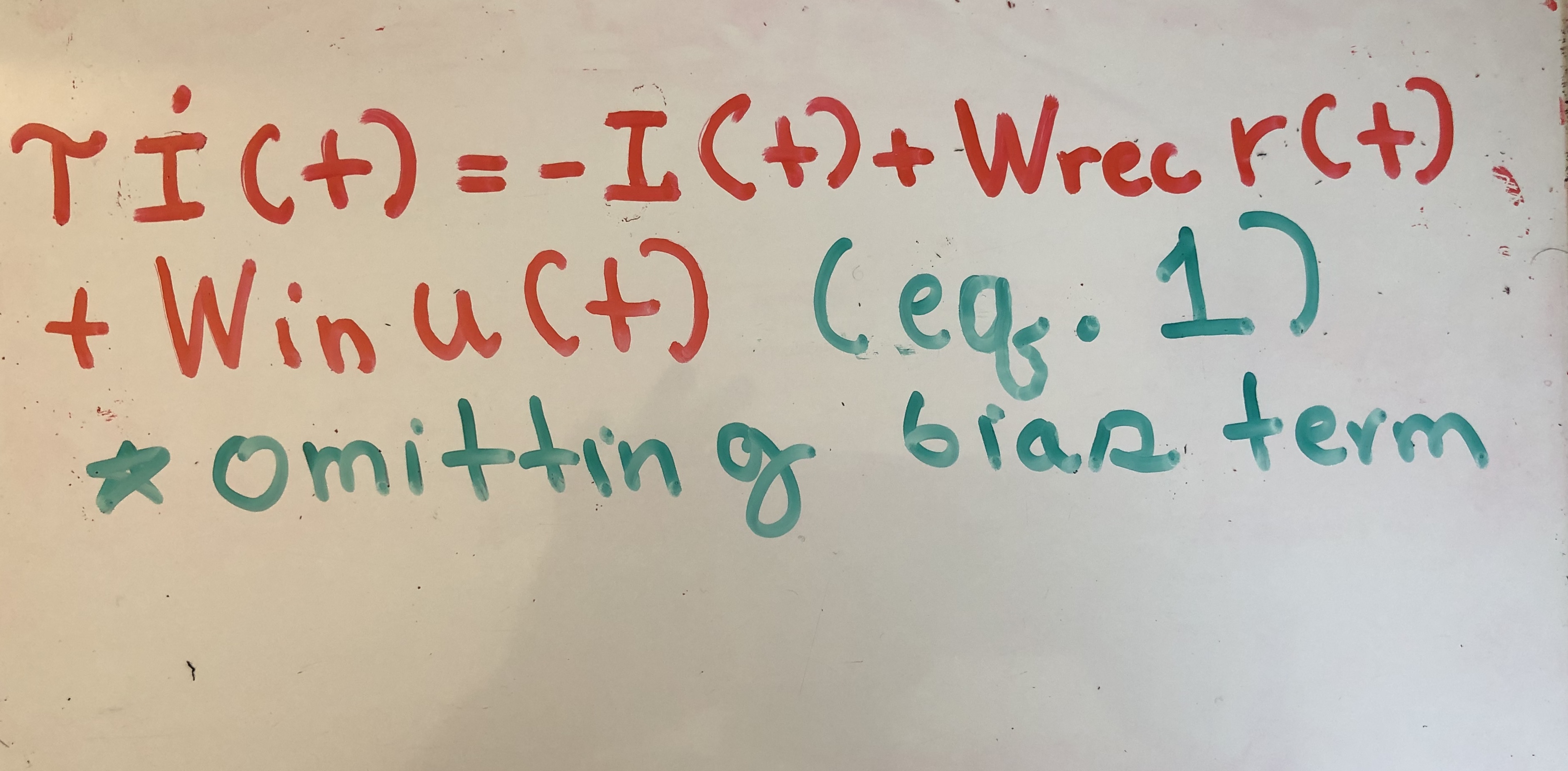
In this equation, i(t) represents the RNN hidden state. r(t) is equal to f(i(t)), where f() represents a nonlinear function, and u(t) is our input. In essence, what this equation is telling us is that our RNN hidden state evolves through time according to a matrix transformation of the previous hidden state and the input. That makes sense. You should update your state according to new, incoming information as well as information from the previous state. However, what never made sense to me was the -i(t) term. Why do you subtract your previous hidden state? Also, where does the time constant tau come from?

Then, I read a paper titled “Adaptive Time Scales in Recurrent Neural Networks”, written by Silvan Quax, Michele D’asaro, and Marcel A.J. van Gerven. The authors beautifully motivate the RNN equations and provide a satisfying explanation for each term, including the -x(t) term and the time constant.

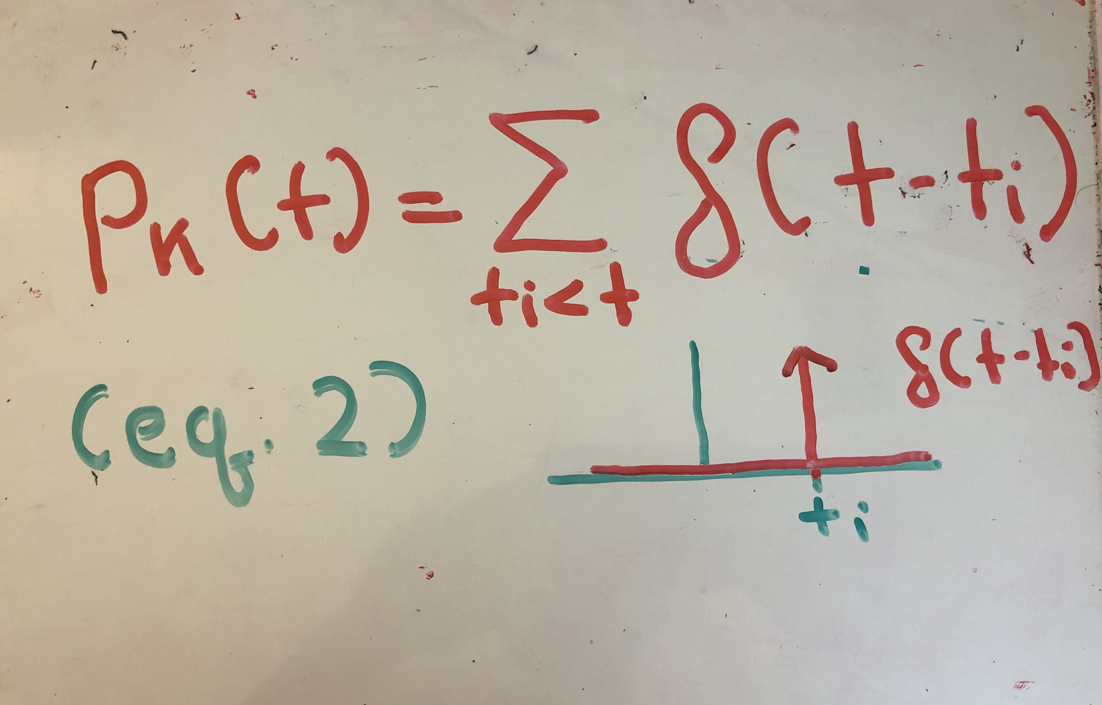
The authors start by first modeling a neural spiking activity with the impulse response function. The impulse response function shoots to infinity at time t=ti (approximating an action potential), and otherwise is 0.

Next, they model the synaptic current that a neuron receives through the following formula:

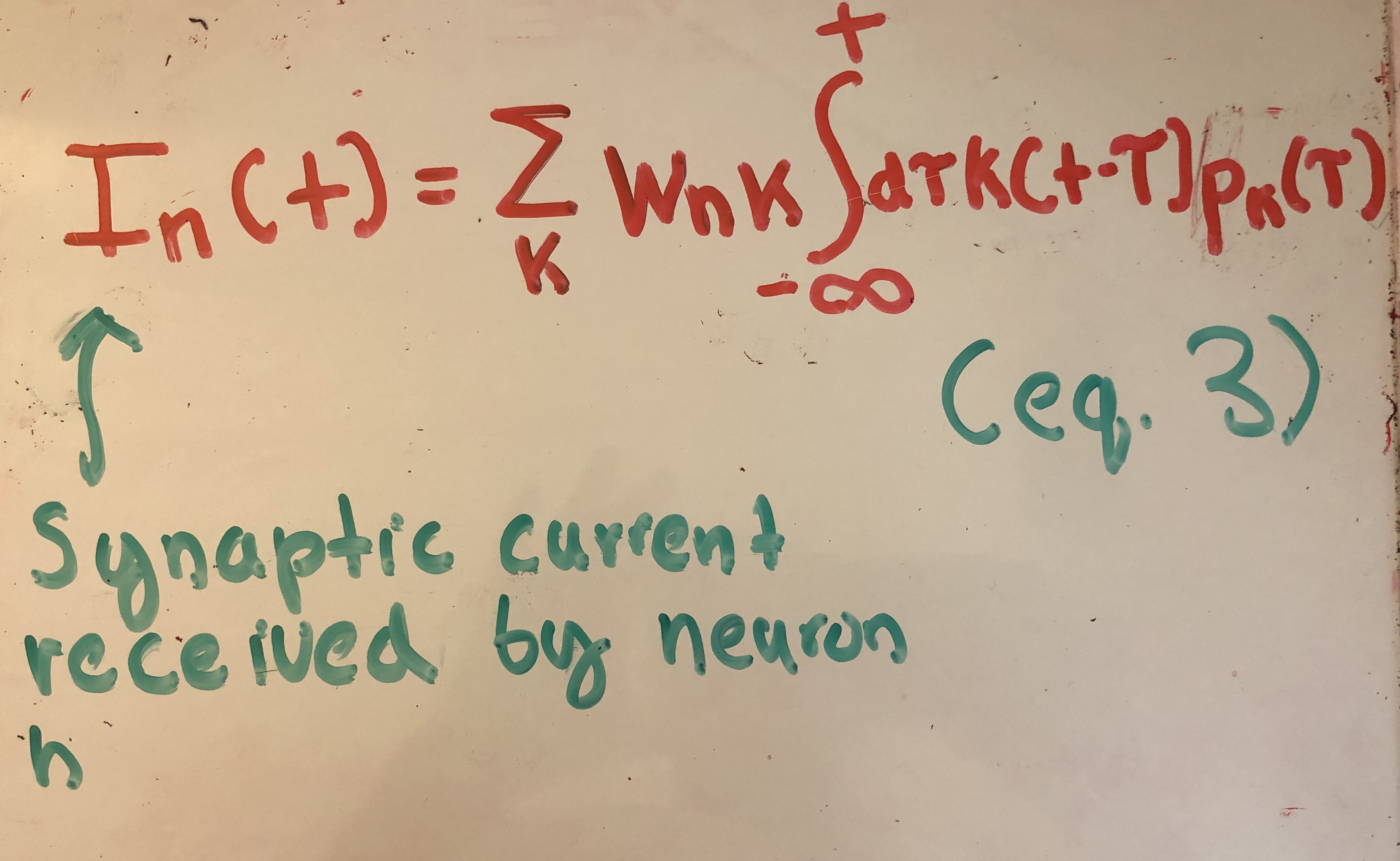
Here, wnk represents the strength of the synaptic weight connection fron neuron k to neuron n. K() is a function which approximates the transformation of an action potential, from neuron k, to the the amount of synaptic current the postsynaptic neuron receives (neuron n). K() is modeled by an exponential kernel in this paper.

The mathematics behind the choice for K() is somewhat beyond the scope of this article, but the underlying intuition is the following. If we assume that a neuron is firing at a constant rate with period T, then the value of the firing rate averaged over T should be 1/T. Working through the calculus we get the requirement that our kernel choice should integrate to 1. The exponential kernel satisfies this property, and also acts as a low-pass filter for the impulse response, jumping up in activity and then slowly decaying. This models synaptic currents in biology well.

Recurrent neural networks, in their standard form, are rate based models. This means that rather than representing individual spike times, RNNs represent a rate code. There is exciting research, by scientists like Chris Eliasmith and many others, on spiking-based models. Howerver, we’ll focus on the more traditional rate based models for now.

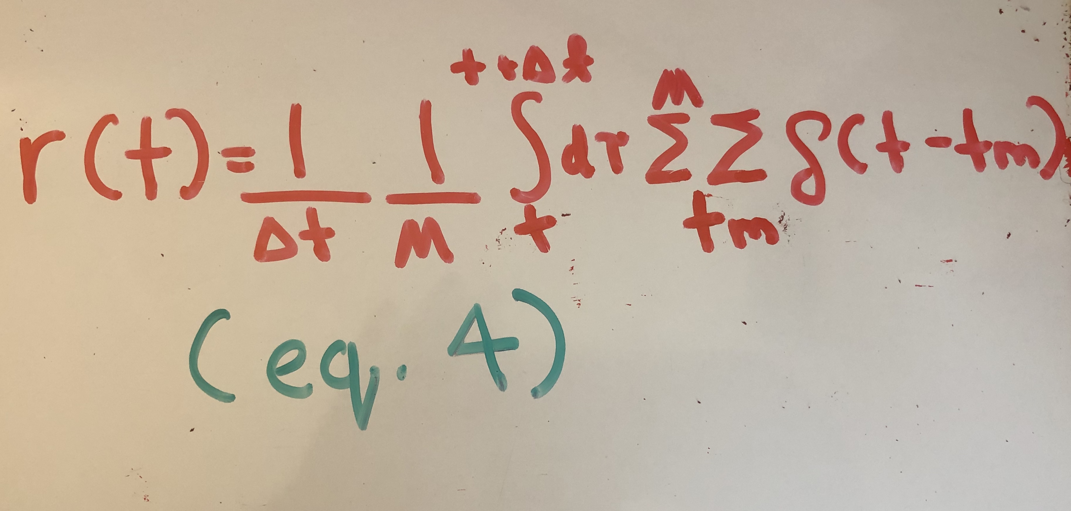
A rate code counts the number of spikes produced by M neurons over a small time interval. It can be expressed through equation (4).

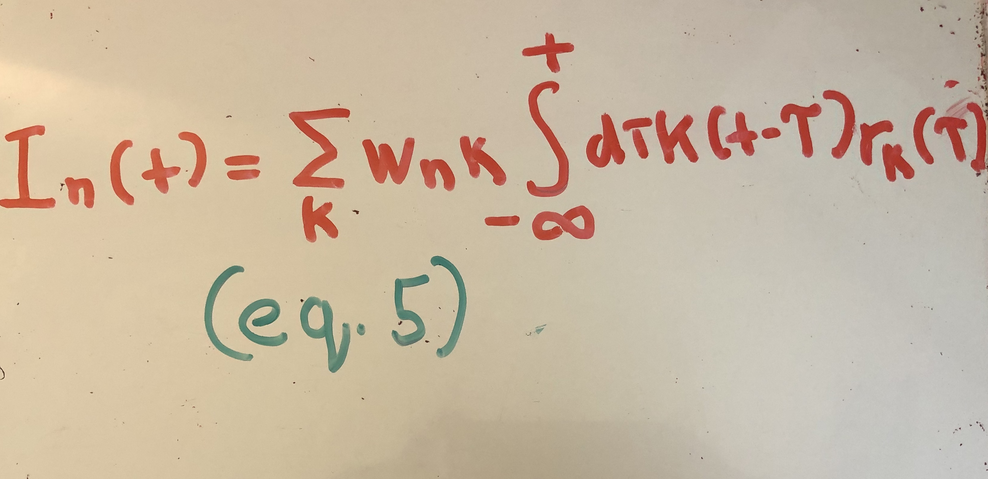
The authors replace the spike train term in equation (2) with the rate code equation. Equation (5) now expresses the synaptic current received by neuron n.

We are finally ready to see how this translates to equation (1). Quax. et. al take the derivative of the synpatic current. I’m going to gloss over this step, but the end result is written in equation (6).

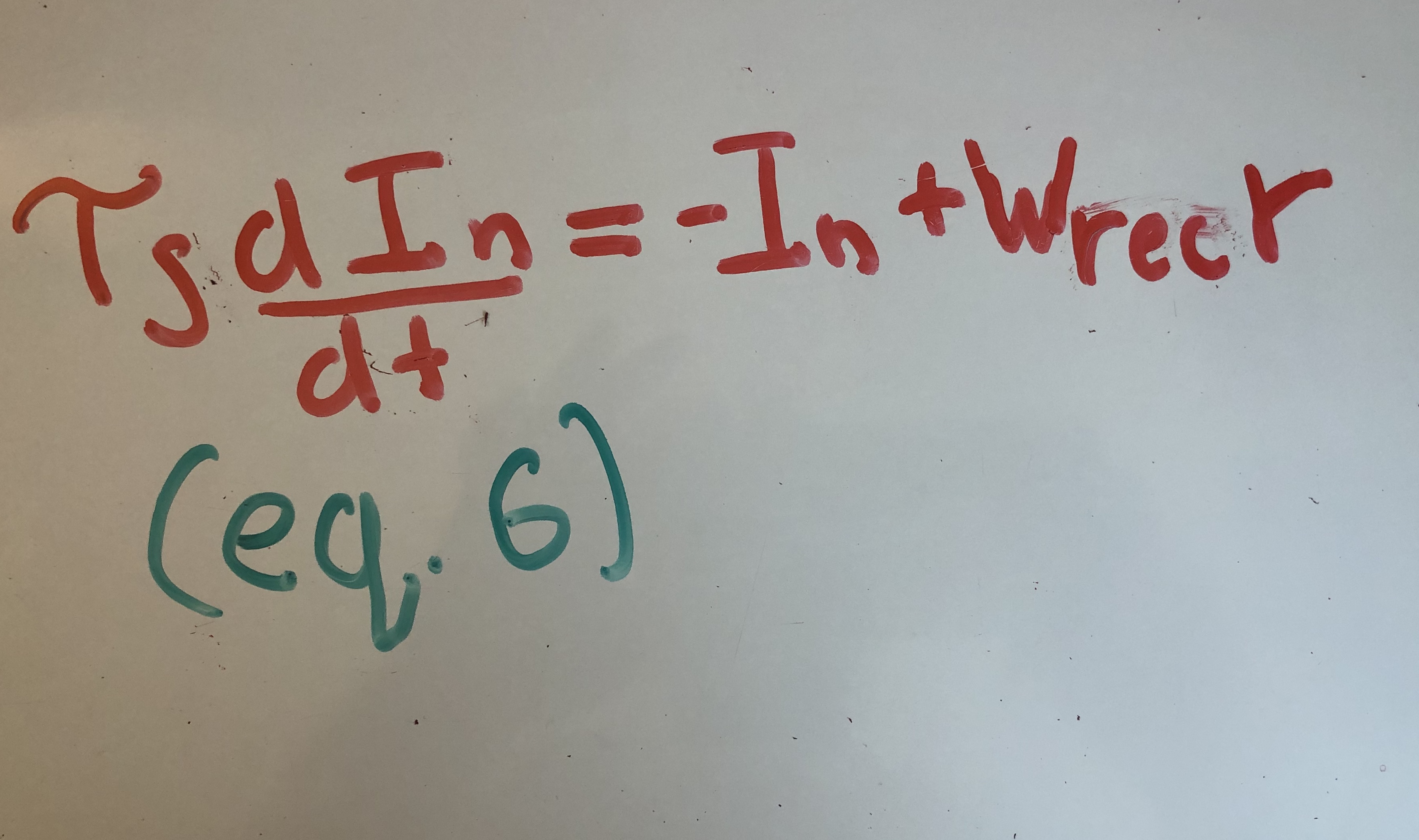
Here, we can see that the time constant in equation (1) arises from the exponential kernel. Also, subtracting the previous hidden state naturally emerges from taking the derivative of the well-motivated equation (5).

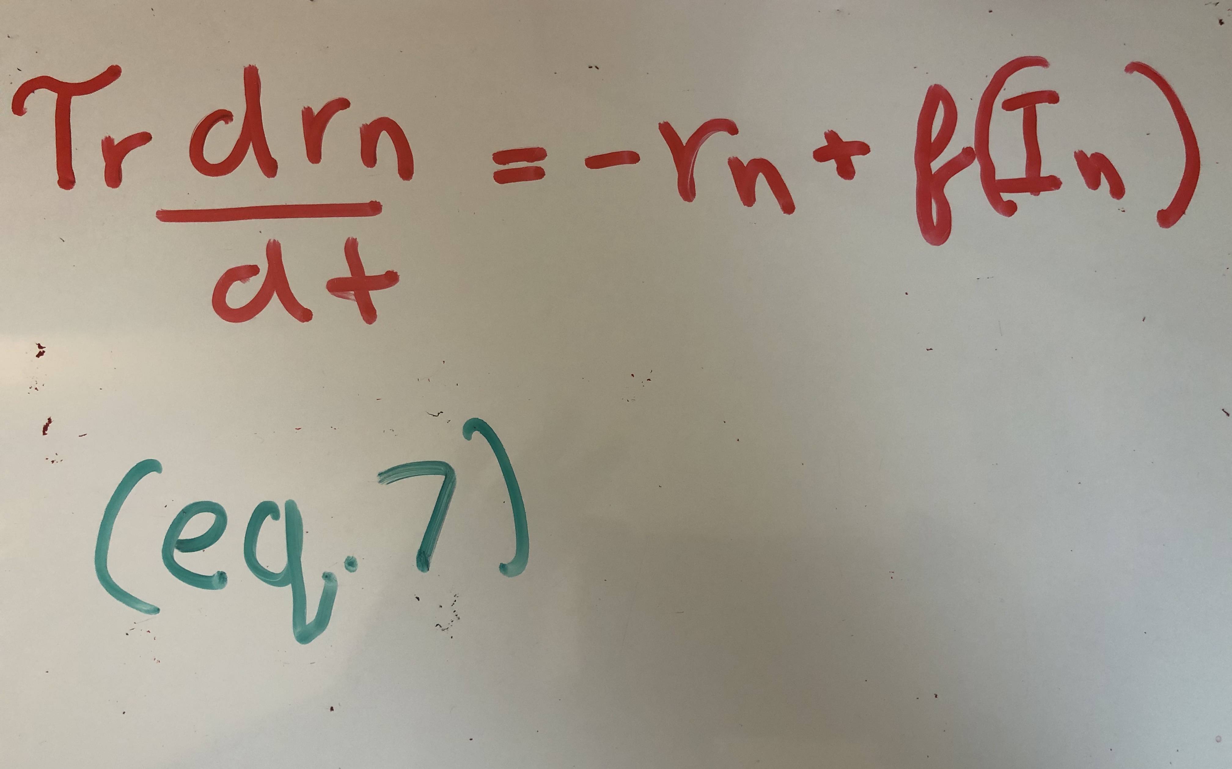
In biology, the membrance capacitance and resistance make it so that neural firing does not immediately follow the current. Quax. et. al model the delay in firing rate by adding a second equation to model the delay in firing rate.

Quax et. al then use Euler’s approximation to convert these continuous time differential equations into discrete hidden state updates. They also add an in an input term, resulting in equation (8).

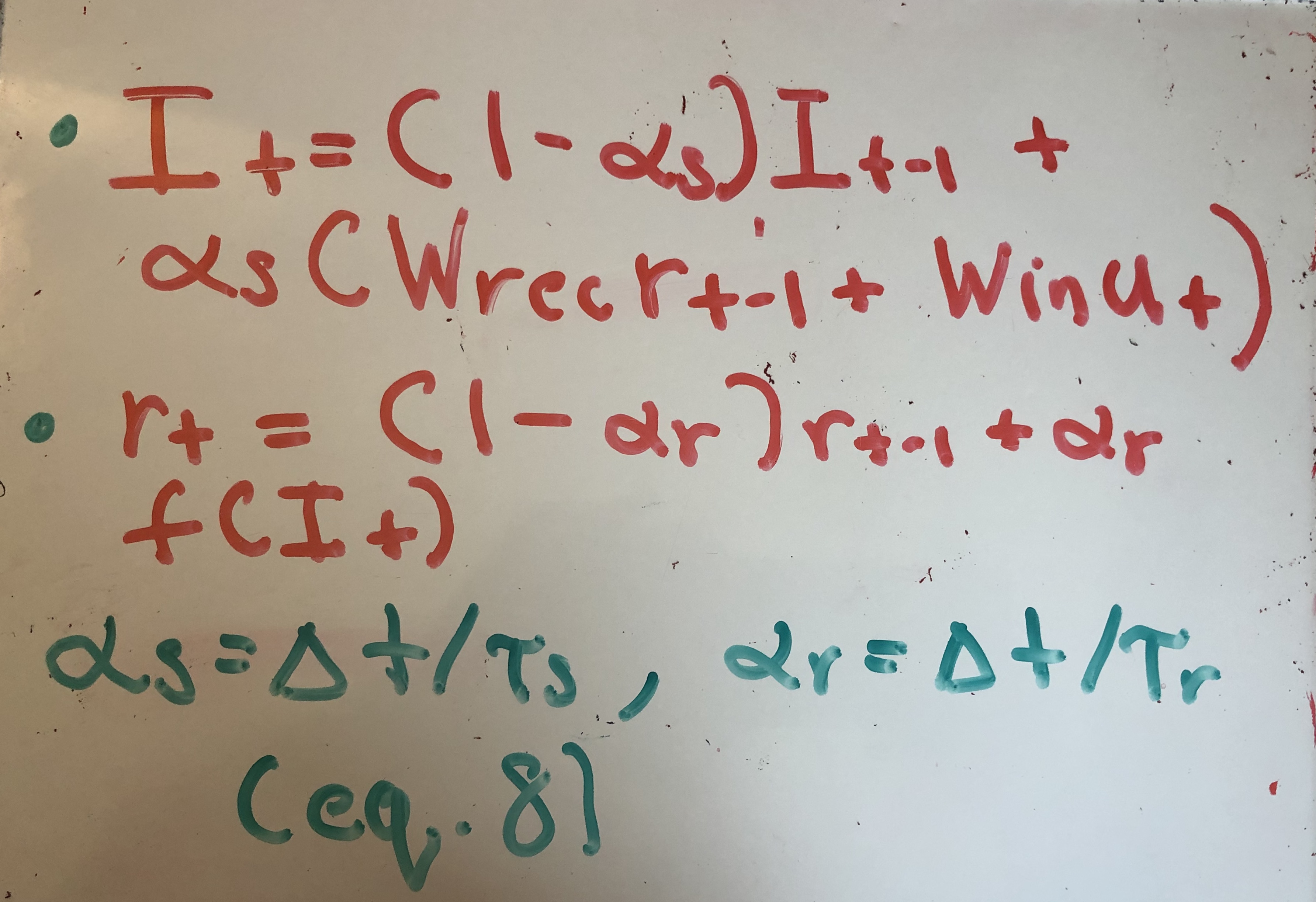
In the machine learning community, the membrane time constants are typically ignored and set to 1. Doing so bring us to equation (1), except now in discrete time domain.

We’ve now come full circle, and hopefully this article helped you gain a better intuition behind the RNN hidden state update equation.